
Lesson 7: Hyper-connections and why they blow up
Part 1 changed the attention. Part 2 turns to the backbone, and it starts with the smallest piece of a Transformer block: the "+" that adds a layer's output to its input. This lesson covers the plain residual connection, the hyper-connection that widens it, and the reason hyper-connections become unstable when many layers are stacked. The repair is lesson 8.
Source: the mHC paper (arXiv 2512.24880), sections 1, 3.1 and 3.2, tables 1, 2, 4 and 5, and section 5.4 for the reported gains; the DeepSeek-V4 report (arXiv 2606.19348), section 2.2, paragraph "Standard Hyper-Connections", and section 4.2.1 for the sizes. Hyper-connections are taken as the mHC paper presents them. The original Hyper-Connections paper was not read. Every number in the worked example comes from lesson07_check.py in this folder.
1. What Part 1 left open
In lessons 5 and 6 the toy replaced a whole layer by a fixed step: one layer pass moved the hidden state of a token by that token's row of D. For "day" in our sentence "The next day is bright and" the row is [0.5, 0, 0, 0], so the state [2, 1, 0, 0] became [3, 1, 0, 0] after two layers.
That step hides an addition. A layer does not output the new hidden state. It outputs a change, and the block adds the change to what came in. This is the "+" in figure 1.4 of the book, and the book counts two of them in every block, one around the attention and one around the feed-forward network. The addition is called a residual connection, and the hidden state that travels up the stack through all the additions is called the residual stream.
The DeepSeek-V4 report replaces this addition with something that has learned weights. To see what is gained and what goes wrong, we first look at what the plain addition does over several layers.
2. The residual connection over four layers
The mHC paper writes one layer as:
x_(l+1) = x_l + F(x_l)
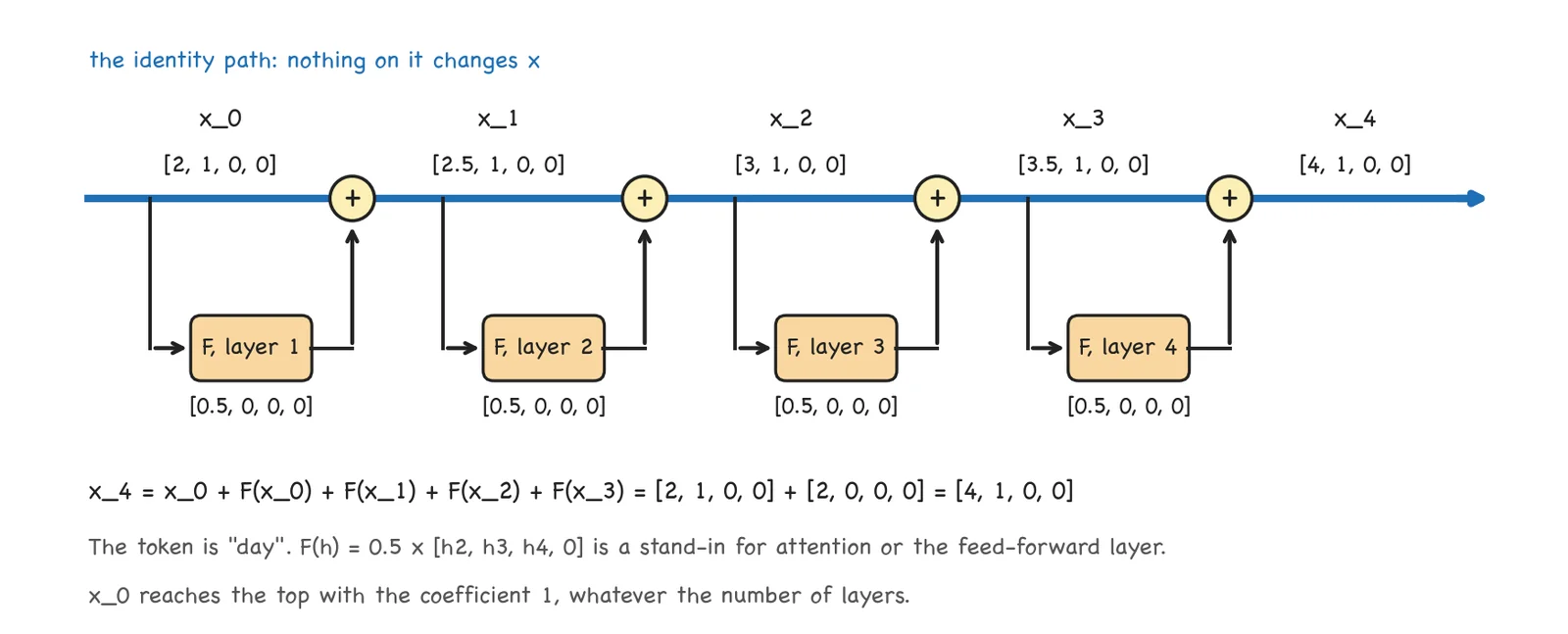
x_l is the hidden state that enters layer l, with C numbers, and F is the layer: attention, or the feed-forward network. The toy needs an F that we can compute by hand, so I chose a stand-in that has nothing to do with attention: F(h) = 0.5 x [h2, h3, h4, 0]. For "day" it returns [0.5, 0, 0, 0], the step of lessons 5 and 6 for this token.
Four layers give four additions:
layer    x_l              F(x_l)            x_l + F(x_l)
1        [2,   1, 0, 0]   [0.5, 0, 0, 0]    [2.5, 1, 0, 0]
2        [2.5, 1, 0, 0]   [0.5, 0, 0, 0]    [3,   1, 0, 0]
3        [3,   1, 0, 0]   [0.5, 0, 0, 0]    [3.5, 1, 0, 0]
4        [3.5, 1, 0, 0]   [0.5, 0, 0, 0]    [4,   1, 0, 0]
If we substitute each line into the next, the four layers collapse into one sum. The paper gives it for any pair of layers l and L:
x_L = x_l + F(x_l) + F(x_(l+1)) + ... + F(x_(L-1))

x_4 = [2, 1, 0, 0] + [2, 0, 0, 0] = [4, 1, 0, 0]
The first term is the point of the design. x_0 appears in x_4 exactly as it entered, with nothing multiplied onto it. The paper says the signal of the shallower layer reaches the deeper layer without any modification. Figure 7.1 draws this as a straight line, the identity path, with the layers attached on the side. The same holds on the way back: the gradient at x_4 reaches x_0 along that line unchanged. The paper credits this identity mapping with keeping the training of large models stable.
Without the "+", the toy state would be [0.5, 0, 0, 0] after one layer and [0, 0, 0, 0] after two. Every layer would have to reproduce everything it wants to keep.
3. Attempt 1: a larger hidden size
The residual stream is the only place where a layer can leave information for the layers above it, and it has C numbers per token. Suppose we want it to carry more.
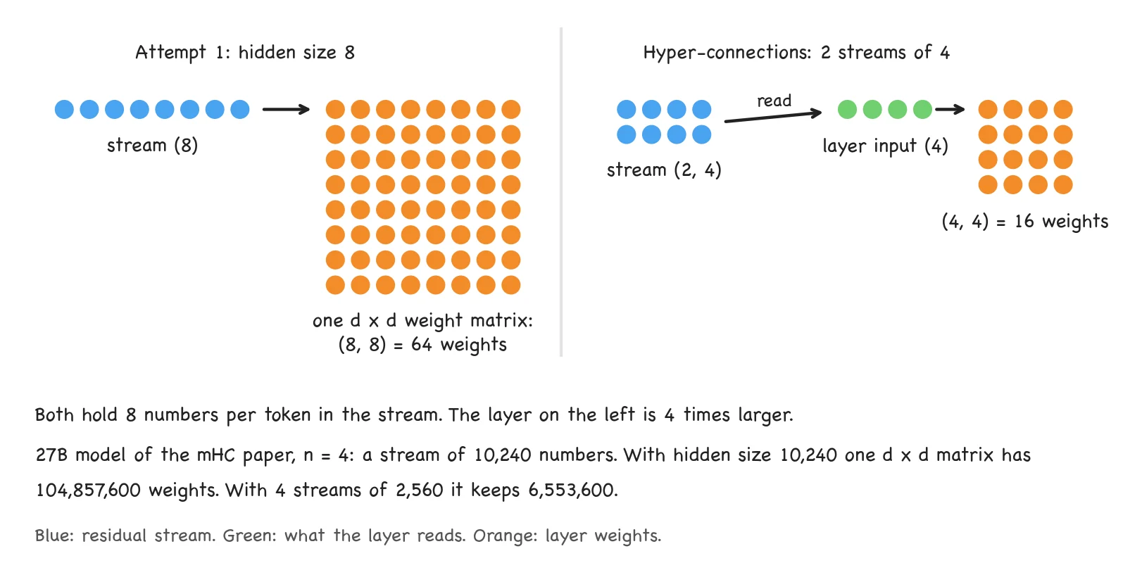
The simplest idea is to raise the hidden size. That makes every layer larger too, because the layers read and write vectors of that size. A weight matrix of shape (d, d) has 16 weights in the toy with d = 4 and 64 with d = 8. At the size of the 27B model in the mHC paper, with d = 2560, a stream four times wider means d = 10,240, and one such matrix grows from 6,553,600 weights to 104,857,600, a factor of 16.
What we want is a wider stream with the layers left at their size, the right side of figure 7.2.
4. Hyper-connections
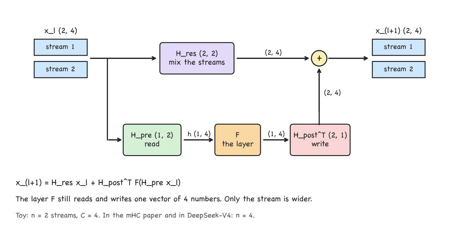
Hyper-connections (HC) keep n streams side by side. The hidden state of a token becomes a matrix x_l with shape (n, C): n rows, which we will call streams, of C numbers each. The paper calls n the expansion rate. The layer F still takes one vector of C numbers and returns one, so three small learned mappings connect the two. The single-layer equation of the paper is:
x_(l+1) = H_res x_l + H_post^T F(H_pre x_l)
H_pre, shape (1, n), reads. It forms a weighted sum of thenstreams, and that sum is the layer's input:(1, n) x (n, C) → (1, C).H_post, shape (1, n), writes. Its transpose copies the layer's output into every stream, each with its own weight:(n, 1) x (1, C) → (n, C).H_res, shape (n, n), mixes. It replaces every stream by a weighted sum of all the streams:(n, n) x (n, C) → (n, C).
Each layer has its own three mappings. Figure 7.3 shows where they sit. The V4 report gives the same equation with the names A_l for the input mapping, B_l for the residual one and C_l for the output one, and it writes n_hc for n.
| Parameter | Symbol | Toy | mHC paper, 27B model | DeepSeek-V4-Pro |
|---|---|---|---|---|
| Hidden size | C (d in the V4 report) | 4 | 2560 | 7168 |
| Streams | n (n_hc) | 2 | 4 | 4 |
| Stream of one token | (n, C) | (2, 4) | (4, 2560) | (4, 7168) |
| Layers | 4 | 30 | 61 |
5. Walkthrough: one layer
Neither source says how the stream is filled at the bottom of the network. In the toy both streams start as copies of "day". The mapping values are mine, chosen for easy arithmetic:
x_0 (2, 4)           H_pre (1, 2)     H_post (1, 2)     H_res (2, 2)
[ 2   1   0   0 ]    [ 0.5   0.5 ]    [ 1   0.5 ]       [ 1.1   0.2 ]
[ 2   1   0   0 ]                                       [ 0.1   0.9 ]
Step 1: read. H_pre (1, 2) x x_0 (2, 4) → h (1, 4)
h = 0.5 x [2, 1, 0, 0] + 0.5 x [2, 1, 0, 0] = [2, 1, 0, 0]
Step 2: the layer. F(h) = 0.5 x [1, 0, 0, 0] = [0.5, 0, 0, 0]
Step 3: write. H_post^T (2, 1) x F(h) (1, 4) → (2, 4)
stream 1:   1   x [0.5, 0, 0, 0] = [0.5,  0, 0, 0]
stream 2:   0.5 x [0.5, 0, 0, 0] = [0.25, 0, 0, 0]
Step 4: mix. H_res (2, 2) x x_0 (2, 4) → (2, 4)
stream 1:   1.1 x [2, 1, 0, 0] + 0.2 x [2, 1, 0, 0] = [2.6, 1.3, 0, 0]
stream 2:   0.1 x [2, 1, 0, 0] + 0.9 x [2, 1, 0, 0] = [2,   1,   0, 0]
Step 5: add.
x_1 (2, 4)
[ 3.1    1.3   0   0 ]
[ 2.25   1     0   0 ]
Figure 7.4 shows the five steps. The two streams now differ, so layer 2 reads a real mixture: 0.5 x [3.1, 1.3, 0, 0] + 0.5 x [2.25, 1, 0, 0] = [2.675, 1.15, 0, 0].
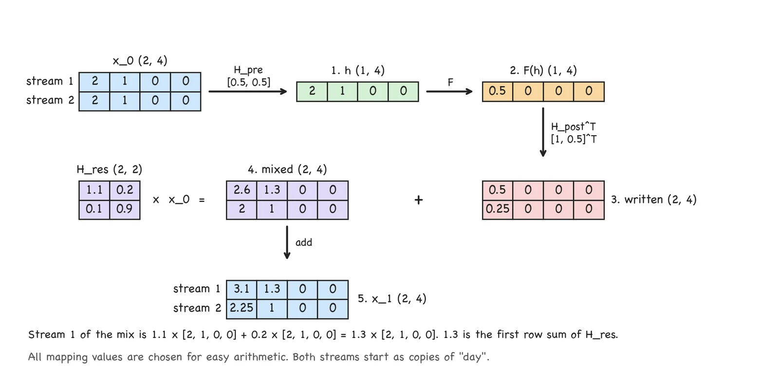
Step 4 deserves a second look. Both streams held the same vector, and stream 1 came out 1.3 times larger. The factor is the sum of the first row of H_res, 1.1 + 0.2. In a residual connection that factor is 1.
6. Four layers: the residual mappings multiply
We now run four layers with two settings.
(a) Fixed mappings. For its ablation, the paper fixes a disabled mapping to uniform weights of 1/n for H_pre, to ones for H_post and to the identity matrix for H_res. With these three, the toy gives [4, 1, 0, 0] in both streams, the result of section 2. The two streams are two copies of the residual stack.
(b) The walkthrough mappings in every layer.
after layer    stream 1                    stream 2
1              [3.1,    1.3,    0, 0]      [2.25,   1,      0, 0]
2              [4.435,  1.63,   0, 0]      [2.6225, 1.03,   0, 0]
3              [6.068,  1.999,  0, 0]      [3.1363, 1.09,   0, 0]
4              [8.0743, 2.4169, 0, 0]      [3.8156, 1.1809, 0, 0]
The second number of each stream is the one to watch. This F never writes to that position, so in a residual stack it stays at 1. Here it reaches 2.4169 in stream 1, and only H_res has touched it.
The unrolled form explains where the number comes from. The paper gives it as the counterpart of the sum in section 2:
x_L = (H_res_(L-1) x ... x H_res_l) x_l + the layer outputs, each multiplied by the H_res of the layers above it
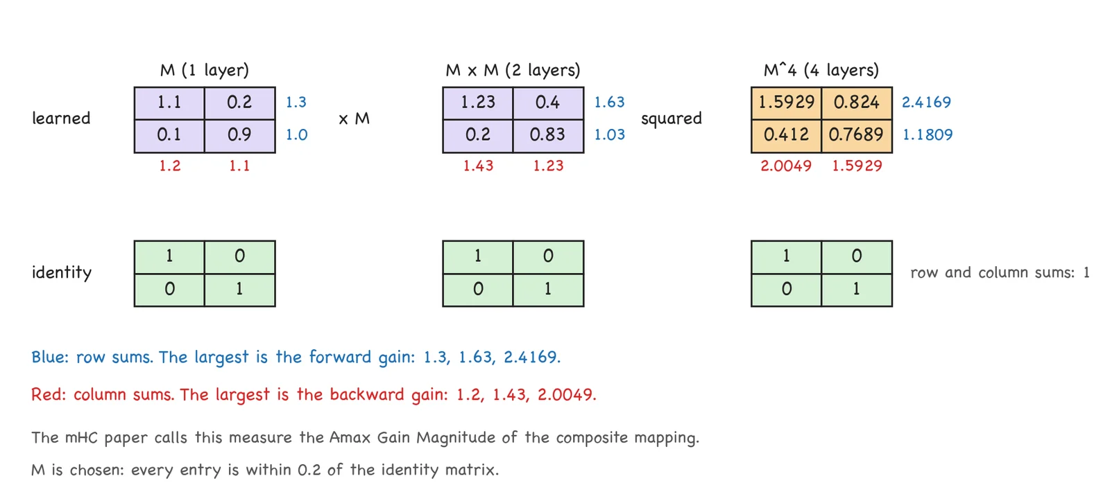
The term that carried x_0 unchanged now carries a product of matrices. With our matrix M in all four layers the product is M x M x M x M, which we compute by squaring twice:
M               M x M              M^4
[ 1.1   0.2 ]   [ 1.23   0.4  ]    [ 1.5929   0.824  ]
[ 0.1   0.9 ]   [ 0.2    0.83 ]    [ 0.412    0.7689 ]
The first row of M^4 sums to 2.4169, the number we just saw in stream 1. The second row sums to 1.1809, the number in stream 2.
The mHC paper measures this with what it calls the Amax Gain Magnitude of the product, which it names the composite mapping. The forward gain is the largest absolute row sum, the worst case for how much the product can enlarge the signal. The backward gain is the largest absolute column sum, because on the way back the gradient is multiplied by the same matrices transposed. For M^4 the forward gain is 2.4169 and the backward gain is 2.0049 (figure 7.5). The script confirms the second number with autograd: a gradient of ones at x_4 arrives at x_0 as 2.0049 in stream 1 and 1.5929 in stream 2. For four identity matrices both gains are 1.
7. Sixty layers
The 27B model of the paper has 30 layers, and its figure 3 unrolls each of them into two, attention and the feed-forward network. By our count that makes 60 residual mappings in one product. The script multiplies 60 of ours:
| Layers multiplied | Identity | M, forward | M, backward | Rows and columns sum to 0.95 |
|---|---|---|---|---|
| 1 | 1 | 1.3 | 1.2 | 0.95 |
| 4 | 1 | 2.4169 | 2.0049 | 0.8145 |
| 16 | 1 | 17.58 | 13.87 | 0.4401 |
| 30 | 1 | 164.69 | 129.89 | 0.2146 |
| 60 | 1 | 19,856 | 15,660 | 0.0461 |
No entry of M is further than 0.2 from the identity, and after 60 layers the product enlarges the signal by a factor of 19,856. Once the growth has settled it is a factor of 1.1732 per layer. The last column shows the opposite case with a matrix that has 0.9 on the diagonal and 0.05 elsewhere: the signal shrinks to 0.0461 of its size. Run through the whole toy with F included, the second number of stream 1 is 19,856 after 60 layers, where setting (a) leaves it at 1.
Using the same M in all 60 layers is a hard case, because every layer pushes in the same direction. So the script also draws a different matrix for each layer, the identity plus Gaussian noise of standard deviation 0.1 on every entry, 1,000 times. The forward gain after 60 layers has a median of 1.821, and 90 percent of the runs fall between 0.596 and 5.50. The largest is 18.7 and the smallest 0.1354. With noise of 0.2 the range between the same percentiles is 0.193 to 20.26, and the largest run reaches 254.8. Deviations without a common direction partly cancel, yet nothing holds the product at 1. Figure 7.6 plots all of these cases.
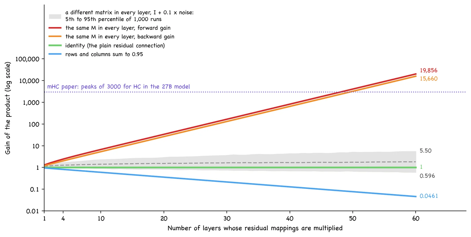
The paper reports the same effect in a real model. In its 27B model with HC, the gain of the composite mapping shows "peaks of 3000" (section 3.1, figure 3), averaged over the tokens of one sequence, and the training loss of that model surges around step 12,000, together with an unstable gradient norm. For scale, a constant factor per layer that reaches 3000 in 60 layers is 1.1428. The V4 report states the same in one sentence: training with standard HC frequently shows numerical instability when many layers are stacked, which hinders scaling it.
8. Why the plain residual connection is safe
In the terms of this lesson, a residual connection is a hyper-connection with one stream whose three mappings are the number 1. Its product over 60 layers is 1 x 1 x ... x 1 = 1. The 1 is a constant of the architecture and not a weight, so training cannot move it.
A residual stack still changes the hidden state, and it does so by addition. In the toy, 60 layers take "day" from [2, 1, 0, 0] to [32, 1, 0, 0]: sixty steps of 0.5.
HC replaced the constant by a learned matrix in every layer. Equation 3 of the paper places no condition on H_res, so nothing ties the product to the identity. The paper's diagnosis is that the composite mapping no longer preserves the global mean of the features, which leads to unbounded amplification or attenuation of the signal in both directions.
9. What hyper-connections give in return
The papers give two reasons to want the wider stream. The V4 report says that HC decouples the width of the residual stream from the hidden size of the layers, which is the goal of section 3. The mHC paper says that the layers can now be connected in many more ways while the cost of each layer in floating-point operations stays the same.
The paper also shows results. On its 27B models, HC is ahead of the residual baseline on all eight benchmarks of table 4: 48.9 against 43.8 on BBH, 53.2 against 46.7 on GSM8K, and 63.0 against 59.0 on MMLU. In the ablation of table 1, learning all three mappings lowers the loss by 0.027, and the text attributes the largest part of that to H_res. The mapping that helps the most is the one whose product is unbounded.
10. What hyper-connections cost
| Toy | mHC paper, 27B model | |
|---|---|---|
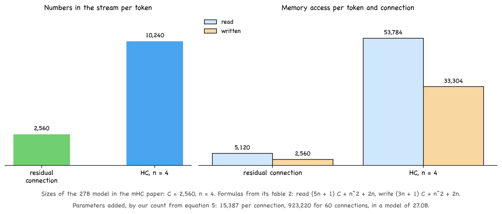
| Numbers in the stream per token: C → n x C | 4 → 8 | 2,560 → 10,240 |
| Entries of the three mappings of one layer: n² + 2n | 8 | 24 |
| Parameters that generate them, per connection: (n + 2) C + n² + 2n + 3 | 27 | 15,387 |
| Connections | 4 | 60 |
| Parameters added in total | 108 | 923,220, in a model of 27.0B |
| Numbers read per token and connection: 2C → (5n + 1) C + n² + 2n | 8 → 52 | 5,120 → 53,784 |
| Numbers written: C → (3n + 1) C + n² + 2n | 4 → 36 | 2,560 → 33,304 |
The read and write formulas are those of table 2 in the paper, which counts memory access and leaves out F. The parameter rows are our count from the shapes in the paper's equation 5, covered in section 12. The paper itself gives no parameter count and only calls the overhead of the mappings negligible.
The cost is in memory traffic. One connection reads 10.5 times as many numbers as a residual connection and writes 13.0 times as many (figure 7.7). The paper adds that the intermediate activations enlarge GPU memory use during training, and that pipeline parallelism has to send n times as much between stages. At the sizes of V4-Pro the stream of one token grows from 7,168 to 28,672 numbers.
11. A hyper-connection in code
The listing has the two functions that lesson07_check.py uses for sections 5 to 7.
import torch

def hc_layer(x, H_pre, H_post, H_res):
    h = H_pre @ x                                #A
    out = F(h)                                   #B
    return H_res @ x + H_post.T @ out            #C

def gains(P):
    fwd = P.abs().sum(dim=1).max().item()        #D
    bwd = P.abs().sum(dim=0).max().item()        #E
    return fwd, bwd
#A Read: (1, n) x (n, C) gives the layer input (1, C).
#B The layer itself. It never sees more than one vector of C numbers.
#C Mix the streams with H_res and add the layer output, written to each stream with its weight in H_post.
#D Forward gain of a product P of residual mappings: the largest absolute row sum.
#E Backward gain: the largest absolute column sum.
12. What the real model adds
- Mappings that depend on the input. In the toy the mappings are fixed numbers. In HC as the paper presents it (equation 5), each mapping is a learned bias plus a part computed from the current stream: the stream is normalized with RMSNorm, projected by a learned matrix, passed through tanh and scaled by a learned factor that starts small. The projections have shapes (1, C) for
H_preandH_postand (n, C) forH_res. Every token therefore gets its ownH_resin every layer. - Four streams. The paper uses
n= 4 in all its models, and V4-Pro and V4-Flash setn_hcto 4. - DeepSeek-V4 does not use plain HC. It uses the constrained form of lesson 8.
Not published in the two sources: how the token embedding becomes n streams and how the streams become one vector before the output head; a parameter count for HC; the gains of single layers as numbers, since the paper shows them only as curves; the layer range on the axis of its figure 3; and which sublayers carry a connection in V4. The HTML of table 1 did not let us read which row belongs to which mapping, so we rely on the text for the statement about H_res.
13. What is still open
- HC performs better than the residual connection in the paper's 27B experiments, and its residual mapping is both the most useful part and the unstable one. Removing
H_reswould give up most of the gain. - The instability grows with depth. The paper measured it in a model of 30 layers, and V4-Pro has 61.
- The identity matrix is the one setting we know to be safe, and it mixes nothing.
What is missing is a set of matrices that can mix the streams and whose products can never amplify, however many are multiplied. The mHC paper finds it in the doubly stochastic matrices, in which every row and every column sums to 1, and it reports a gain of about 1.6 where HC reached 3000. Lesson 8 builds these matrices and the Sinkhorn-Knopp iteration that produces them.