
Lesson 11: Muon and Newton-Schulz iterations in DeepSeek-V4
Lesson 10 ended on the rule that turns a gradient into an update. This lesson opens Part 3 with Muon, the optimizer that DeepSeek-V4 uses for most of its weights, and the Newton-Schulz iteration inside it.
Source: the DeepSeek-V4 report (arXiv 2606.19348), section 2.4 with its Algorithm 1, section 3.4.1, and the optimizer settings of section 4.2.2; the Kimi K2 report (arXiv 2507.20534) for one sentence on QK-Clip. Every number in the worked examples comes from lesson11_check.py in this folder.
1. What AdamW leaves open
Chapter 6 of the book trains its model with AdamW. AdamW treats a weight matrix as a list of separate numbers. Every entry has its own running averages and its own step size, and no entry knows which row or column it sits in.
The model uses the matrix as a whole: a vector goes in and a vector comes out. V4 trains most of its matrices with an optimizer that reads the gradient the same way. The report's stated reasons are faster convergence and improved training stability, and it publishes no comparison with AdamW. We start from a gradient small enough to take apart by hand.
2. A gradient with two unequal directions
Our toy weight matrix W is 2 × 2, and so is its gradient G. The values are chosen for easy arithmetic.
G = [ 4.848   3.536 ]
    [ 6.364   4.848 ]
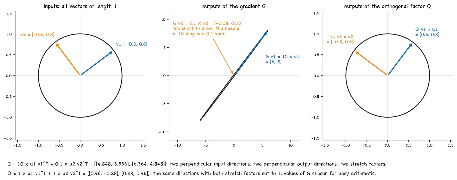
The four entries look alike. What the matrix does shows when we feed it two input vectors of length 1 that are perpendicular to each other, v1 = [0.8, 0.6] and v2 = [-0.6, 0.8].
G v1 = [ 6, 8 ]          = 10  × u1      u1 = [ 0.6, 0.8 ]
G v2 = [ -0.08, 0.06 ]   = 0.1 × u2      u2 = [ -0.8, 0.6 ]
The outputs u1 and u2 also have length 1 and are perpendicular. So G stretches the input direction v1 by 10 and puts it out along u1, and it shrinks v2 to a tenth and puts it out along u2.
Every matrix can be described this way: perpendicular input directions, perpendicular output directions, and one stretch factor for each pair. The description is called the singular value decomposition, SVD for short, and the stretch factors are the singular values. Written as a sum:
G = 10 × u1 v1ᵀ + 0.1 × u2 v2ᵀ

u1 v1ᵀ = [ 0.48   0.36 ]      u2 v2ᵀ = [  0.48   -0.64 ]
         [ 0.64   0.48 ]               [ -0.36    0.48 ]
We call u1 v1ᵀ direction 1 and u2 v2ᵀ direction 2. Figure 11.1 draws what G does to a circle of inputs.
3. Attempt 1: a plain SGD step
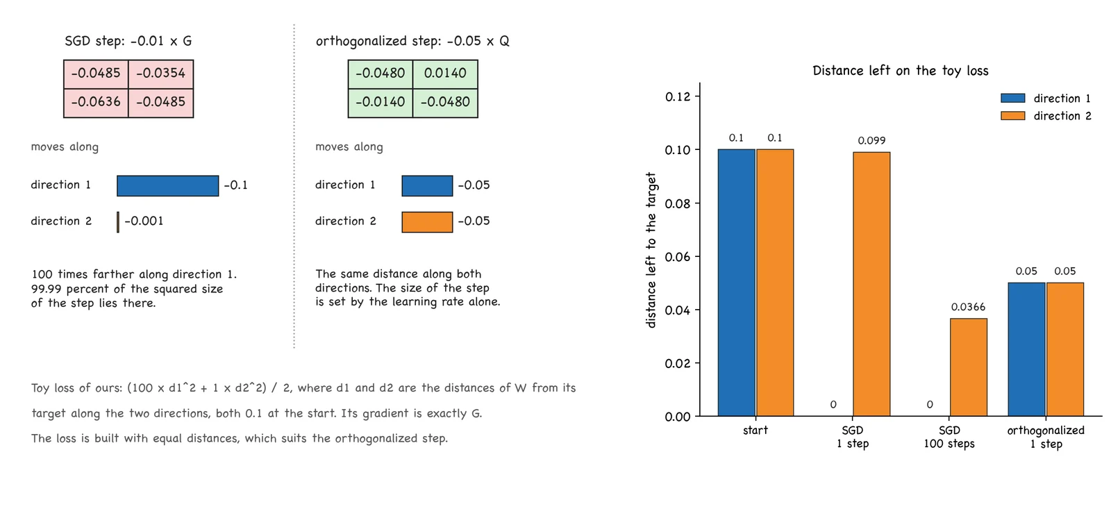
SGD subtracts the gradient times a learning rate, W ← W - lr × G. With lr = 0.01 the step is -0.1 along direction 1 and -0.001 along direction 2. The step moves 100 times farther along direction 1.
A small singular value does not mean that direction 2 is finished. A gradient is also small where the loss is flat. Take a loss of our own in which W is 0.1 away from its target along both directions, and the loss curves 100 times more sharply along direction 1:
loss = (100 × d1² + 1 × d2²) / 2          d1 = d2 = 0.1
gradient along each direction = curvature × distance = 10 and 0.1
This is exactly G. SGD is stable here only for lr below 2 / 100 = 0.02. With lr = 0.01 one step closes direction 1 completely and leaves direction 2 at 0.099. After 100 steps direction 2 stands at 0.0366. The step size that direction 1 allows is far too small for direction 2.
4. Attempt 2: set both stretch factors to 1
Suppose we keep the two directions of G and replace both stretch factors by 1.
Q = 1 × u1 v1ᵀ + 1 × u2 v2ᵀ = [ 0.96   -0.28 ]
                               [ 0.28    0.96 ]
A matrix whose stretch factors are all 1 is called orthogonal. It turns vectors and leaves their lengths alone: Q v1 = u1 and Q v2 = u2. Its columns have length 1 and are perpendicular. To orthogonalize G means to replace it by this Q.
A step -lr × Q moves by lr along both directions. On the loss of section 3, one step with lr = 0.05 takes both distances from 0.1 to 0.05 (figure 11.2). We built that loss with equal distances, which suits this update perfectly, and the report does not argue from such an example.
To get Q, the check script calls torch.linalg.svd, which returns the singular values 10 and 0.1 with their directions, and multiplies the directions back together. V4-Flash has, by our count, 33,153 expert matrices with 2,048 singular values each, and every one needs a new Q at every training step. The report does not discuss the SVD. The usual objection is that SVD routines proceed in many small steps that each wait for the one before, which a GPU does poorly. We want Q from the operation a GPU does best, the matrix multiplication.
5. Newton-Schulz: matrix multiplications only
The Newton-Schulz iteration starts from X = G divided by a number, and repeats one formula:
X ← a X + b (X Xᵀ) X + c (X Xᵀ)² X
To see what one step does, write X as its two directions, X = s1 × u1 v1ᵀ + s2 × u2 v2ᵀ. In the product (X Xᵀ) X the vectors meet in pairs, a v with a v or a u with a u. A vector paired with itself gives 1 and paired with the other gives 0, because the vectors have length 1 and are perpendicular. All mixed terms vanish:
(X Xᵀ) X  = s1³ × u1 v1ᵀ + s2³ × u2 v2ᵀ
(X Xᵀ)² X = s1⁵ × u1 v1ᵀ + s2⁵ × u2 v2ᵀ
So a step leaves both directions where they are and replaces each stretch factor s by
p(s) = a s + b s³ + c s⁵
The matrix iteration is a scalar iteration running on every singular value at once, and no SVD is ever computed. In the script, one matrix step and the polynomial agree to 3.9 × 10^-16.
The coefficients must make repeated use of p send every stretch factor to 1. The report runs 10 steps with two sets:
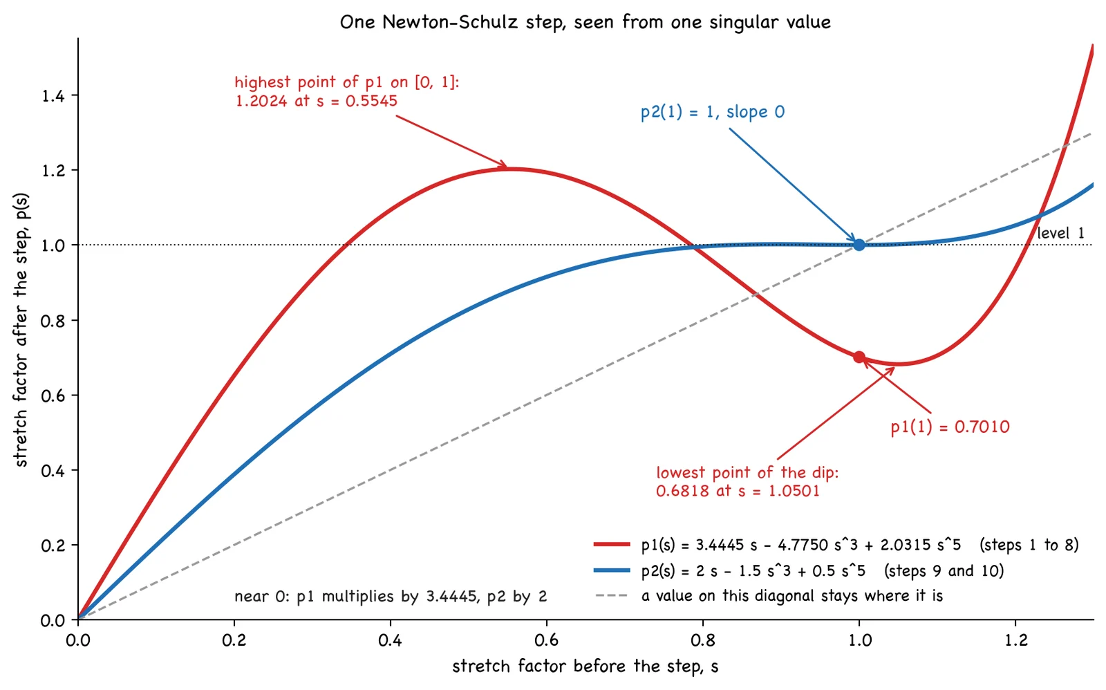
steps 1 to 8:     p1(s) = 3.4445 s - 4.7750 s³ + 2.0315 s⁵
steps 9 and 10:   p2(s) = 2 s - 1.5 s³ + 0.5 s⁵
Before the first step the matrix is divided by its Frobenius norm, the square root of the sum of its squared entries. The report says this ensures that the largest singular value does not exceed 1. For G the norm is √(10² + 0.1²) = 10.0005, so the two singular values start at 1.0000 and 0.0100.
6. The iteration by hand
One value through p1, starting at 0.5:
3.4445 × 0.5 = 1.7223      4.7750 × 0.5³ = 0.5969      2.0315 × 0.5⁵ = 0.0635
p1(0.5) = 1.7223 - 0.5969 + 0.0635 = 1.1889
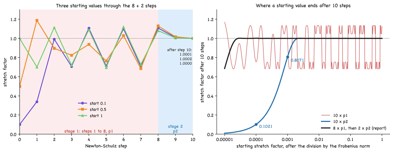
Three starting values through all 10 steps:
step   start 0.1   start 0.5   start 1.0
0      0.1000      0.5000      1.0000
1      0.3397      1.1889      0.7010      stage 1
2      0.9921      0.8962      1.1136
3      0.7071      0.8244      0.7207
4      1.1066      0.9379      1.0900
5      0.7121      0.7654      0.6964
6      1.1006      1.0289      1.1188
7      0.7057      0.6855      0.7277
8      1.1082      1.1306      1.0810
9      1.0106      1.0171      1.0053      stage 2
10     1.0001      1.0002      1.0000
Stage 1 never settles. A value of exactly 1 is sent to p1(1) = 0.7010, and every column keeps bouncing between about 0.69 and 1.13. Stage 2 does settle: p2(1) = 1, and the slope of p2 at 1 is 0, so a value near 1 lands much nearer. Figure 11.3 plots the two polynomials and figure 11.4 the three columns.
7. Why two stages
If p2 settles at 1, why not run it ten times? The answer is in the small starting values.
start     10 × p1    10 × p2    8 + 2
1         1.1253     1.0000     1.0000
0.1       1.0983     1.0000     1.0001
0.01      1.1219     1.0000     1.0000
0.001     0.9881     0.8071     1.0000
0.0001    0.7547     0.1021     1.0020
Close to zero only the first term of a polynomial counts, so p1 multiplies a tiny value by 3.4445 at each step and p2 by 2. Eight steps of p1 lift it 19,816 times, and ten steps of p2 only 1,024 times. Alone, p2 leaves a start of 0.0001 at 0.1021. Alone, p1 lifts everything and ends anywhere between 0.6818 and 1.1344. Together, the eight steps bring every start between 0.001 and 1 into that band, and the two steps of p2 take the band to between 1.0000 and 1.0005.
Small starts are the normal case in a large matrix. A (2048, 4096) matrix has 2,048 singular values, and if all are equal each starts at 1 / √2048 = 0.0221. In an example of ours, half of them are 100 times smaller than the other half. Those start at 0.0003125, ten steps of p2 leave them at 0.3120, and 8 + 2 brings them to 1.0000.
The report gives one clause per stage: the first 8 steps bring the singular values close to 1 quickly, and the last 2 pin them at 1. How the coefficients were found is not published.
8. The matrix iteration on the toy
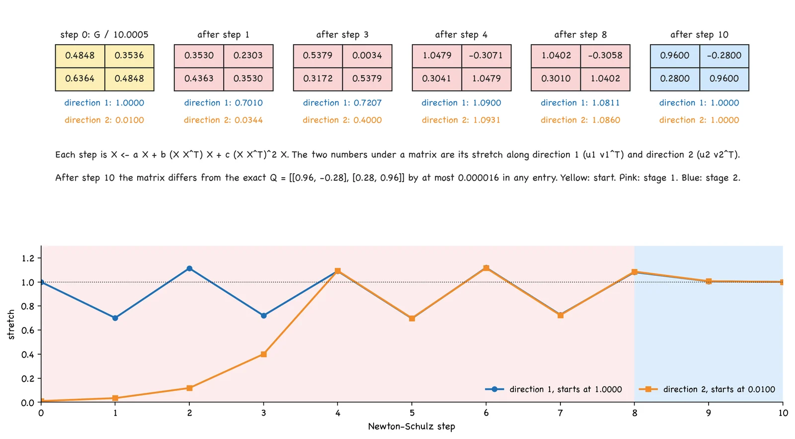
The script now runs the matrix formula on G and reads off the stretch along each direction.
step   direction 1   direction 2      X, first row and second row
0      1.0000        0.0100           [ 0.4848  0.3536 ]   [ 0.6364  0.4848 ]
1      0.7010        0.0344
2      1.1136        0.1184
3      0.7207        0.4000
4      1.0900        1.0931           [ 1.0479 -0.3071 ]   [ 0.3041  1.0479 ]
5      0.6965        0.6989
6      1.1187        1.1160
7      0.7276        0.7239
8      1.0811        1.0860
9      1.0053        1.0061
10     1.0000        1.0000           [ 0.9600 -0.2800 ]   [ 0.2800  0.9600 ]
Direction 2 starts 100 times below direction 1 and is level with it by step 4. Direction 1 starts at 0.99995, so its column differs from the last column of section 6 in the fourth decimal. The result differs from the exact Q by at most 1.6 × 10^-5 in any entry (figure 11.5).
9. One full Muon step
Algorithm 1 of the report applies five lines to each "logically independent" weight matrix W of shape (n, m):
G_t  = gradient of the loss at W_(t-1)
M_t  = μ M_(t-1) + G_t                       momentum
O'_t = HybridNewtonSchulz(μ M_t + G_t)       Nesterov trick, then orthogonalize
O_t  = O'_t × √max(n, m) × γ                 rescale
W_t  = W_(t-1) × (1 - η λ) - η O_t           weight decay and step
Section 4.2.2 gives μ = 0.95, λ = 0.1 and a peak learning rate η of 2.7 × 10^-4 for V4-Flash and 2.0 × 10^-4 for V4-Pro. It also says that the RMS of each update matrix is rescaled to 0.18. RMS is the root mean square, the square root of the mean of the squared entries.
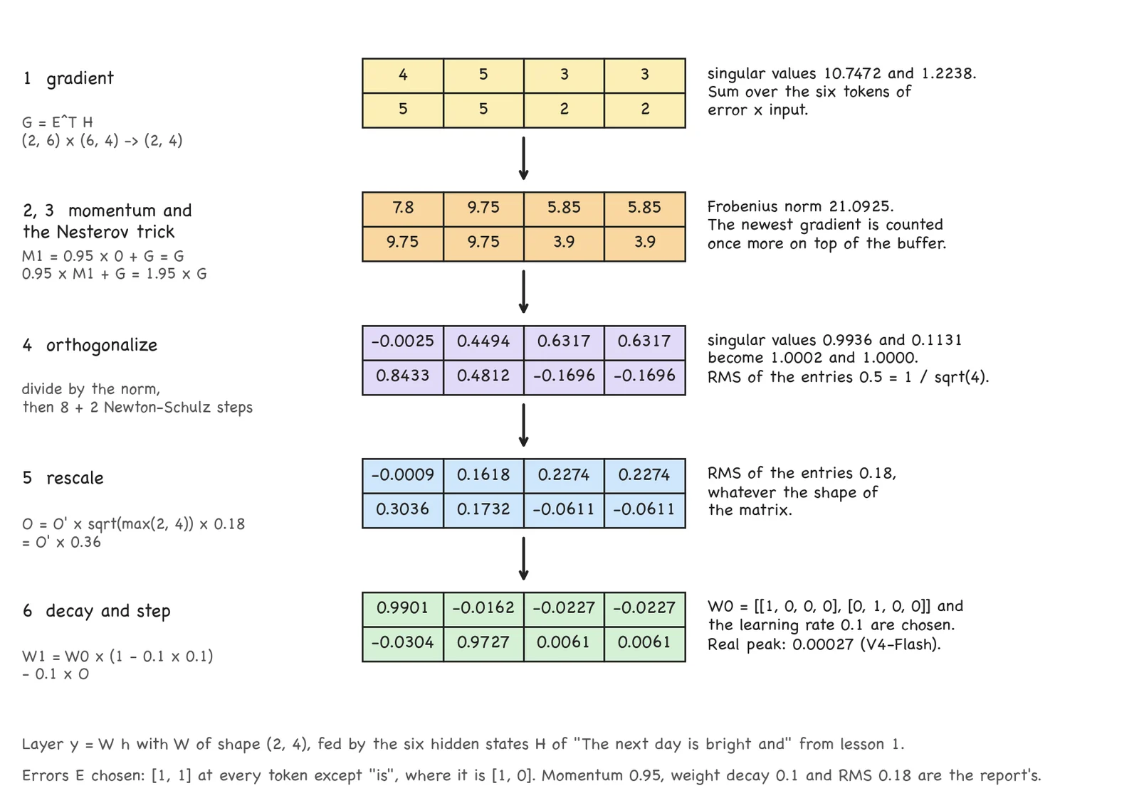
We run the five lines on a layer fed by our sentence, y = W h with W of shape (2, 4) and the hidden states H of lesson 1. As the error at the layer output we choose [1, 1] at every token except "is", where it is [1, 0].
Step 1: the gradient. It is the sum over the six tokens of error times input, Eᵀ H, (2, 6) × (6, 4) → (2, 4).
G = [ 4  5  3  3 ]        singular values 10.7472 and 1.2238
    [ 5  5  2  2 ]
Step 2: momentum. The buffer starts at zero, so M1 = G.
Step 3: the Nesterov trick. Plain momentum would hand on M1. The trick counts the newest gradient once more and hands on 0.95 M1 + G = 1.95 G. At a second step with a gradient G2, the buffer holds 0.95 G + G2 and the matrix handed on is 0.9025 G + 1.95 G2.
Step 4: orthogonalize. Dividing by the Frobenius norm, 21.0925, removes the factor 1.95: the size of the gradient plays no part in the update. The singular values start at 0.9936 and 0.1131 and end at 1.0002 and 1.0000.
O' = [ -0.0025   0.4494   0.6317   0.6317 ]
     [  0.8433   0.4812  -0.1696  -0.1696 ]
This matrix is not square, so it is the two rows that have length 1 and are perpendicular, here to within 0.0002.
Step 5: rescale. O' has two singular values of 1, so its squared entries sum to 2, spread over 8 entries. Its RMS is √(2 / 8) = 0.5, which is 1 / √max(2, 4). Multiplying by √max(n, m) therefore brings the RMS to 1 for any shape, and γ then sets it to γ. On this ground we read the 0.18 of section 4.2.2 as γ, a link the report does not make itself. Its stated purpose for the rescaling is that the hyperparameters of AdamW can be reused.
O = O' × 2 × 0.18 = [ -0.0009   0.1618   0.2274   0.2274 ]      RMS 0.1800
                    [  0.3036   0.1732  -0.0611  -0.0611 ]
Step 6: decay and step. With W0 = [[1, 0, 0, 0], [0, 1, 0, 0]] and a learning rate of 0.1, both chosen, W1 = 0.99 × W0 - 0.1 × O.
W1 = [  0.9901  -0.0162  -0.0227  -0.0227 ]
     [ -0.0304   0.9727   0.0061   0.0061 ]
Figure 11.6 shows the six steps.
10. AdamW and Muon on the same gradient
On its first step on the toy G, AdamW has seen one gradient, so its two bias-corrected averages are G and G², entry by entry. Its update direction is G divided by the square root of G², which is the sign of each entry.
                 first row, second row                along direction 1   along direction 2
gradient G       [ 4.848  3.536 ] [ 6.364  4.848 ]    10                  0.1
AdamW, step 1    [ 1  1 ] [ 1  1 ]                    1.96                -0.04
Muon, O'         [ 0.96  -0.28 ] [ 0.28  0.96 ]       1                   1
AdamW has made the four entries equal in size. As a matrix, though, its update has the singular values 2 and 0, so it moves along a single direction. Muon moves 1 along each direction of G (figure 11.7).
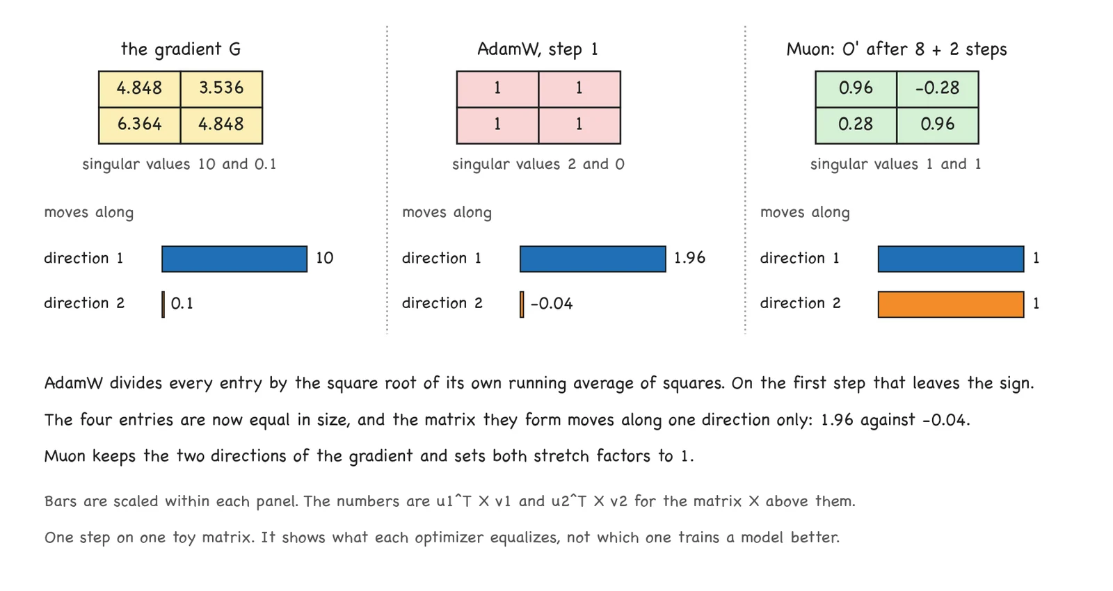
This is one step on one matrix. On later steps the update of AdamW is no longer an exact sign. The table shows what each optimizer equalizes, and it does not show which one trains a model better.
11. What stays with AdamW, and QK-Clip
V4 keeps AdamW for four groups of parameters: the embedding, the prediction head, the static biases and gating factors of mHC from lesson 8, and the weights of all RMSNorm modules. All other modules are updated with Muon. The report gives no reason for the split.
The report also names a technique called QK-Clip, says V4 does not use it, and does not describe it. In the Kimi K2 report, QK-Clip is a step added after the Muon update: when the largest logit of an attention head passes a threshold, the query and key weights of that head are scaled down. V4 does without it because its attention applies RMSNorm directly to the queries and the KV entries, as we saw in lesson 4, and the report says this effectively keeps the logits from exploding.
12. What the orthogonalization costs
Grouped as in the listing of section 13, one Newton-Schulz step is three matrix multiplications: X Xᵀ, its square, and the product with X. Ten steps make 30 for every weight matrix at every training step.
| Toy | Sentence layer | V4-Flash expert matrix | |
|---|---|---|---|
| Shape (n, m) | (2, 2) | (2, 4) | (2048, 4096) |
| Singular values | 2 | 2 | 2,048 |
| Newton-Schulz steps | 8 + 2 | 8 + 2 | 8 + 2 |
| Matrix multiplications per training step | 30 | 30 | 30 |
| Multiply-adds in those 30 | 240 | 400 | 429,496,729,600 |
| √max(n, m) × 0.18 | 0.2546 | 0.36 | 11.52 |
| RMS of the update | 0.18 | 0.18 | 0.18 |
| Momentum, weight decay | 0.95, 0.1 | 0.95, 0.1 | 0.95, 0.1 |
| Learning rate | 0.1 in the script, chosen | 0.1, chosen | peak 2.7 × 10^-4 |
The multiply-adds are our count, with
X Xᵀtaken on the short side. The report does not say whether a tall matrix is transposed first.
Over all 33,153 expert matrices of V4-Flash that is 1.424 × 10^16 multiply-adds per step. The experts' forward pass on a batch of 75.5M tokens costs 5.719 × 10^17 if every layer runs 7 experts per token, so Newton-Schulz adds 2.49 percent by our count.
Section 3.4.1 describes what had to change to run Muon across many GPUs.
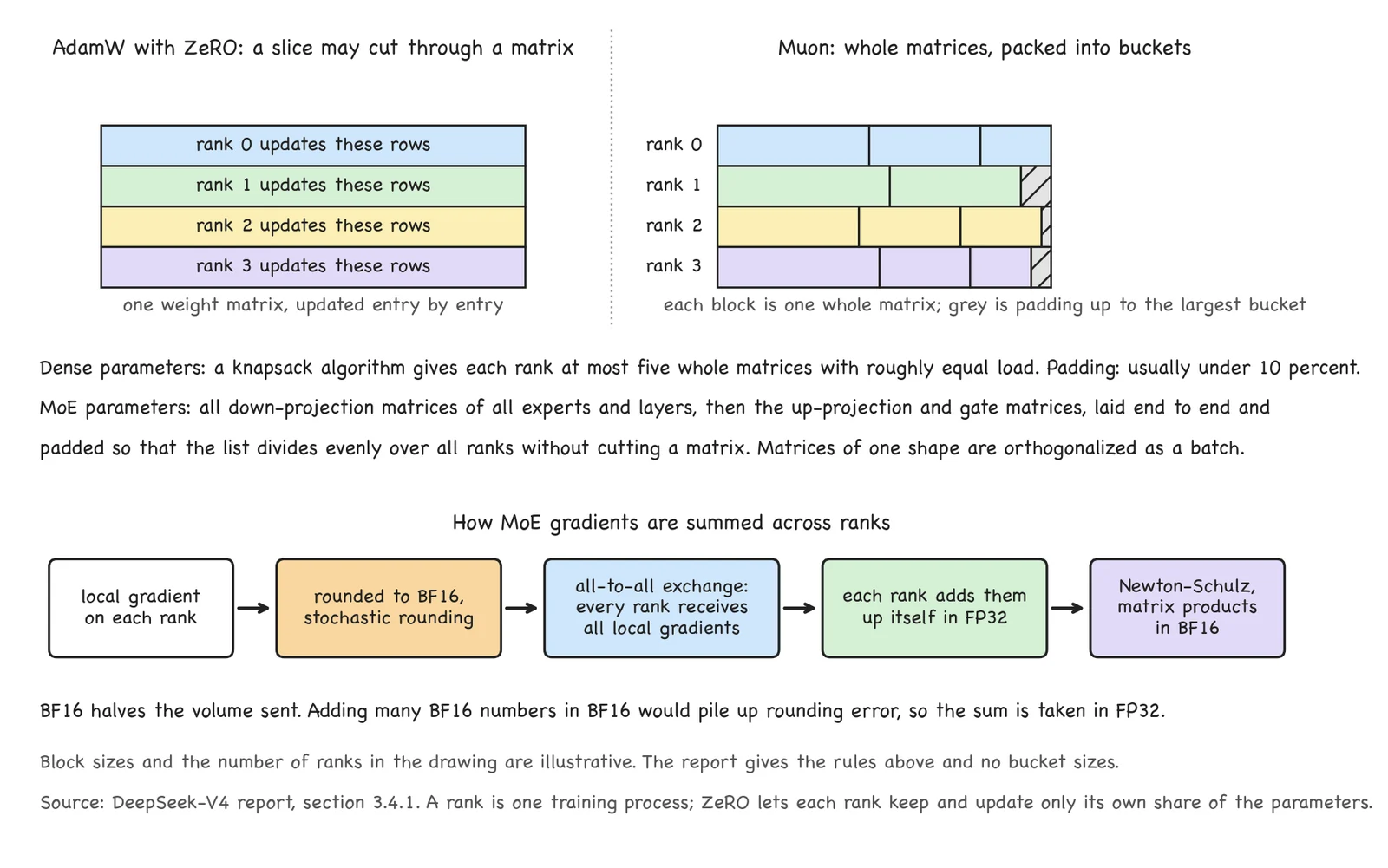
- Whole matrices. ZeRO, the Zero Redundancy Optimizer, is a scheme in which each training process, called a rank, keeps the optimizer state and computes the update for its own slice of the parameters only. AdamW works entry by entry, so a slice may cut through a matrix. Muon needs the whole gradient matrix in one place.
- Dense parameters. A knapsack algorithm assigns whole matrices to ranks with roughly equal loads, and the number of ranks that share them is capped. Each rank's share, its bucket, holds at most five matrices and is padded to the size of the largest bucket, which usually adds less than 10 percent of memory.
- MoE parameters. All down-projection matrices of all experts and layers are laid end to end, then the up-projection and gate matrices, and the list is padded so that it divides evenly over all ranks without cutting a matrix (figure 11.8). On each rank, neighbouring matrices of the same shape are orthogonalized as one batch.
- BF16. The report finds Newton-Schulz stable when its matrix multiplications run in BF16. On our toy, the ten steps in BF16 end at 0.9954 and 0.9954, where FP32 gives 1.0000.
- Gradients. MoE gradients are rounded to BF16, with stochastic rounding, before the ranks exchange them, which halves the volume sent. To keep rounding errors from piling up in a BF16 sum, every rank first receives the local gradients of all the others and then adds them up itself in FP32.
13. Muon in code
import math
import torch

STAGES = [(3.4445, -4.7750, 2.0315)] * 8 + [(2.0, -1.5, 0.5)] * 2

def hybrid_newton_schulz(M):
    X = M / M.norm()                                   #A
    for a, b, c in STAGES:                             #B
        A = X @ X.T                                    #C
        X = a * X + (b * A + c * A @ A) @ X            #D
    return X

def muon_step(W, G, M, lr, mu=0.95, wd=0.1, gamma=0.18):
    M = mu * M + G                                     #E
    O = hybrid_newton_schulz(mu * M + G)               #F
    O = O * math.sqrt(max(W.shape)) * gamma            #G
    W = W * (1 - lr * wd) - lr * O                     #H
    return W, M
#A Divide by the Frobenius norm, so that no singular value exceeds 1.
#B Eight steps with the first coefficients, two with the second.
#C First multiplication: (n, m) × (m, n) → (n, n).
#D Second and third: A times A, then (n, n) × (n, m) → (n, m).
#E The momentum buffer.
#F The Nesterov trick, then the orthogonalization.
#G The RMS of the update becomes gamma for any shape.
#H Weight decay and the step.
14. What the real model adds
- Schedule. V4-Flash warms up linearly over 2,000 steps, holds the peak learning rate for most of training, and decays to a tenth of it on a cosine curve near the end.
- AdamW settings. β1 = 0.9, β2 = 0.95, ε = 10^-20 and a weight decay of 0.1, as for Muon.
Not published: any comparison of Muon with AdamW; the time Muon costs; how the coefficients were found; the reason for the AdamW split.
15. What is still open
- The update throws away the size of the gradient and every difference between its singular values. The report states the benefit and gives no account of why this is safe.
- Ten steps are an approximation. They end within 0.01 of 1 for every start above 2.31 × 10^-5, and smaller singular values are left behind.
- The optimizer already depends on number formats. Newton-Schulz runs in BF16, gradients travel in BF16 and are summed in FP32, and on the toy BF16 alone moved the result from 1.0000 to 0.9954.
The third point is where Part 3 goes next. The book covered FP8, and lessons 3 to 5 met FP4 in the indexer and in the cache. Lesson 12 takes up the formats themselves: FP8, UE8M0 and FP4, and quantization-aware training.