
Lesson 1: DeepSeek Sparse Attention (DSA)
This lesson picks up where chapter 3 of the book ends. It covers the one architectural change in DeepSeek-V3.2: a small scoring module that decides which past tokens the attention layer reads.
Source: the DeepSeek-V3.2 report (arXiv 2512.02556) and the released V3.2-Exp inference code. Every number in the worked example comes from lesson01_check.py in this folder.
1. What MLA left unsolved
In chapter 3, MLA reduced what we store. Instead of a full key and a full value for every head, each past token leaves one latent vector c_kv in the cache, and the cache became about 64 times smaller.
MLA did not reduce how many past tokens we read. When the model predicts the next token, the newest token still compares its query with the cached entry of every earlier token. With 6 tokens in the context, that is 6 comparisons. With 128,000 tokens, it is 128,000 comparisons for a single new token, and each comparison runs through all 128 attention heads. Figure 1.1 shows this for our six-token example.
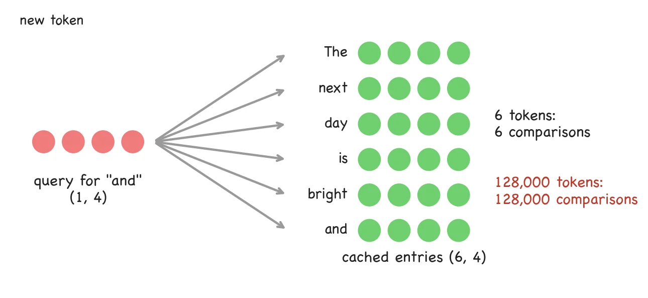
The same holds when the model first reads a long prompt. Token 1 looks at 1 entry, token 2 at 2 entries, and token L at L entries:
pairs = 1 + 2 + ... + L = L x (L + 1) / 2
For L = 128,000 this is 8,192,064,000 query-key pairs in every layer. The cache fits in memory now, but the attention work still grows with the square of the context length.
2. Does a token need every past token?
Let us look at what attention does with all those comparisons. We will reuse the running sentence from the book and extend it by one word:
The next day is bright and → ?
Suppose the attention layer has computed the six scores for the last token, "and". (These are the scaled scores from chapter 3, taken as given here.)
            The    next   day    is     bright  and
score       0.2    0.5    2.0   -1.0    2.4     1.6
exp(score)  1.2214 1.6487 7.3891 0.3679 11.0232 4.9530     sum = 26.6033
weight      0.0459 0.0620 0.2777 0.0138 0.4144  0.1862
Three tokens, "day", "bright" and "and", hold 0.2777 + 0.4144 + 0.1862 = 0.8783 of the total weight. The other three share the remaining 0.1217. Figure 1.2 plots the six weights.
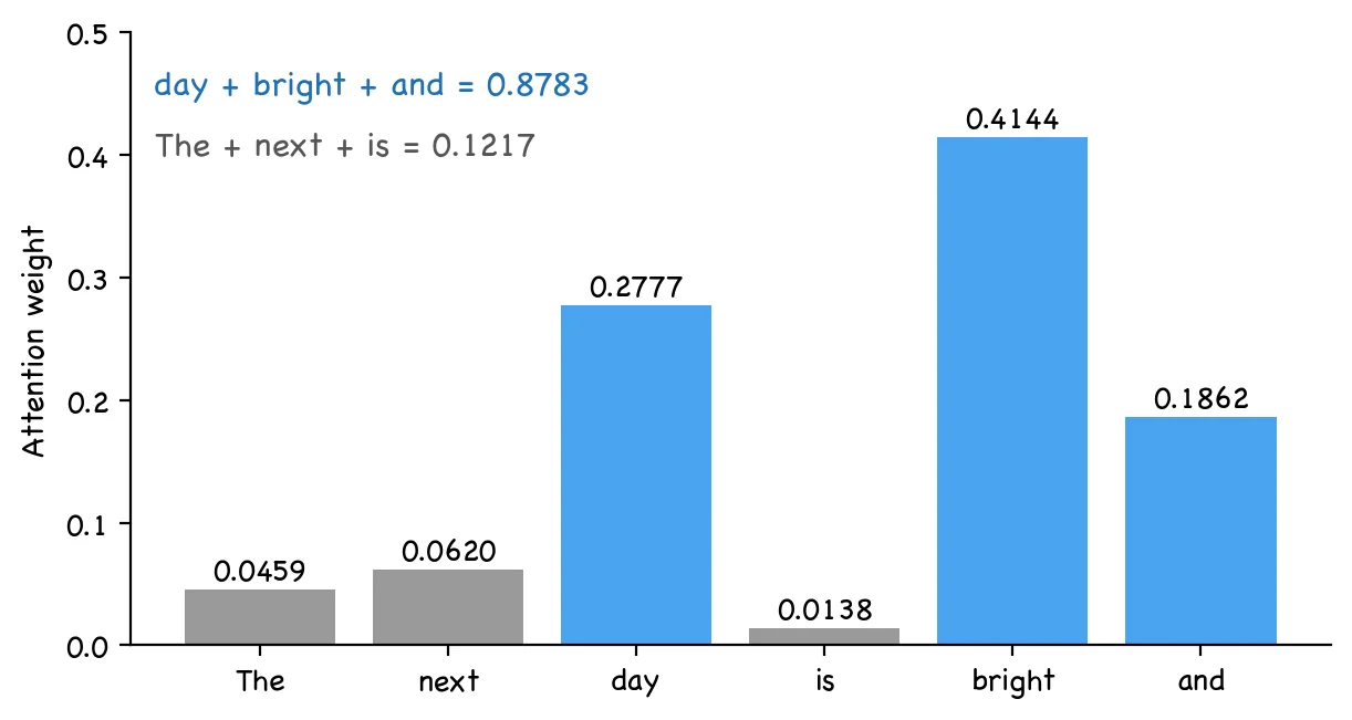
This is a property of softmax. It exponentiates the scores, so a gap of 2 in score becomes a factor of about 7.4 in weight. In a context of 128,000 tokens the effect is much stronger: most tokens receive a weight close to zero, and they contribute almost nothing to the context vector. We are paying for 128,000 comparisons and using a few thousand of them.
3. Attempt 1: compute everything, keep the best
The simplest idea is to compute all six scores, keep the three largest, and run softmax over those three.
This does not help, because the scores are the expensive part. To know which three scores are largest, we first have to compute all six. At real scale we would still compute 128,000 scores for every token and every head, and only skip a small amount of work afterwards.
We need to know which tokens matter before the expensive attention runs.
4. Attempt 2: a cheap scorer that runs first
DeepSeek's answer is a second, much smaller scoring module that runs ahead of the attention layer. The V3.2 report calls it the lightning indexer. Its job is to give a rough relevance score to every past token, cheaply. The top k tokens by that score are passed to the real attention, and the rest are skipped.
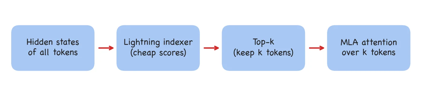
For a query token t and a past token s, the index score from the report is:
I(t, s) = sum over indexer heads j of w(t, j) x ReLU( q(t, j) · k(s) )
There are three ingredients:
k(s): one small key vector for each past tokens.q(t, j): one small query vector for the query tokentin each indexer headj.w(t, j): one number per head, also computed from the query token. It says how much headjcounts for this query.
The indexer is cheaper than the main attention for four reasons. It has fewer heads, each token has a single small key instead of a key per head, it uses ReLU instead of a softmax, and the report says it can run in FP8.
5. The toy setup
| Parameter | Symbol | Toy value | DeepSeek-V3.2 |
|---|---|---|---|
| Context length | L | 6 | up to 128K |
| Hidden size | d_model | 4 | 7168 |
| Indexer heads | H_I | 2 | 64 |
| Indexer head dimension | d_I | 2 | 128 |
| Tokens kept per query | k | 3 | 2048 |
The V3.2 column for the indexer comes from the released inference code (
index_n_heads = 64,index_head_dim = 128,index_topk = 2048). The structure is the same as in the toy; only the sizes differ.
The hidden states entering the layer form the matrix H with shape (6, 4):
           H (6, 4)
The      [  1   0   0   1 ]
next     [  0   1   1   0 ]
day      [  2   1   0   0 ]
is       [ -1   0   1   1 ]
bright   [  1   2   1   0 ]
and      [  1   1   0   1 ]
The indexer has three weight matrices. I chose simple values so that every product can be checked by hand. A trained model learns these.
W_k (4, 2)        W_q (4, 4)            W_w (4, 2)
[ 1  0 ]          [ 1  0  0  0 ]        [ 0.5  0 ]
[ 0  1 ]          [ 0  0  0  1 ]        [ 0    0 ]
[ 0  0 ]          [ 0  0  0  0 ]        [ 0    0 ]
[ 0  0 ]          [ 0  0  0  0 ]        [ 0    1 ]
6. Walkthrough: the lightning indexer
We follow one query token, "and", the newest token in the sequence. Figure 1.4 shows the three projections that steps 1 to 3 carry out.
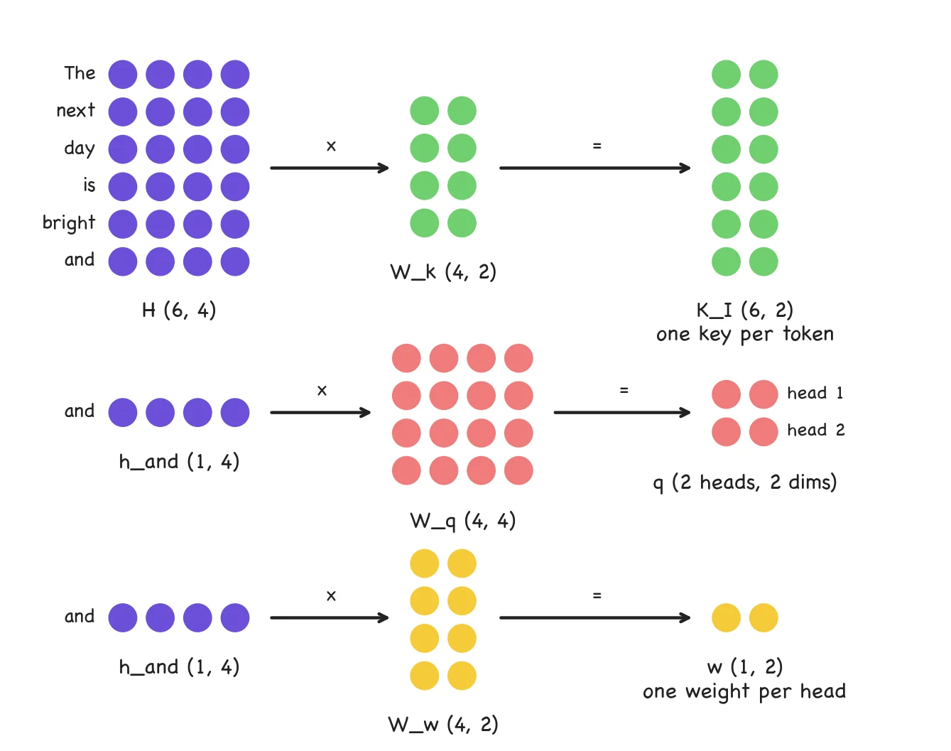
Step 1: one small key per token.
H (6, 4) x W_k (4, 2) → K_I (6, 2)
           K_I (6, 2)
The      [  1   0 ]
next     [  0   1 ]
day      [  2   1 ]
is       [ -1   0 ]
bright   [  1   2 ]
and      [  1   1 ]
For example, the row for "day" is [2, 1, 0, 0] x W_k = [2x1 + 1x0, 2x0 + 1x1] = [2, 1].
These keys are computed once per token and cached, just like c_kv in MLA.
Step 2: the query vectors for "and".
h_and (1, 4) x W_q (4, 4) → (1, 4), then split into 2 heads of 2 dimensions.
[1, 1, 0, 1] x W_q = [1, 0, 0, 1]

head 1:  q1 = [1, 0]
head 2:  q2 = [0, 1]
Step 3: the head weights for "and".
h_and (1, 4) x W_w (4, 2) → w (1, 2)
[1, 1, 0, 1] x W_w = [0.5, 1.0]
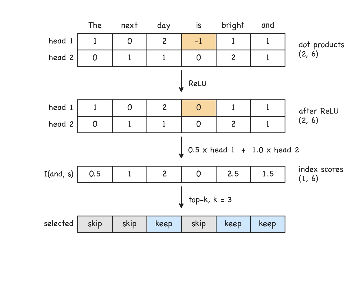
Step 4: dot products, one row per head.
Each head takes the dot product of its query with all six keys: q (2, 2) x K_I transposed (2, 6) → (2, 6).
            The   next   day   is   bright   and
head 1       1     0      2    -1     1       1
head 2       0     1      1     0     2       1
Step 5: ReLU.
ReLU replaces negative numbers with zero. Only one entry changes, "is" in head 1.
            The   next   day   is   bright   and
head 1       1     0      2     0     1       1
head 2       0     1      1     0     2       1
A negative dot product means "this head sees no match". ReLU turns that into a plain zero, so a mismatch in one head cannot cancel a match found by another head.
Step 6: weighted sum over heads.
Multiply the head 1 row by 0.5, the head 2 row by 1.0, and add:
            The   next   day   is   bright   and
0.5 x h1    0.5   0      1.0   0     0.5     0.5
1.0 x h2    0     1.0    1.0   0     2.0     1.0
            ───────────────────────────────────────
I(and, s)   0.5   1.0    2.0   0     2.5     1.5
Step 7: top-k.
With k = 3, the three largest index scores are "bright" (2.5), "day" (2.0) and "and" (1.5). These three tokens are selected. "The", "next" and "is" are skipped. Figure 1.5 collects steps 4 to 7 in one picture.
7. Walkthrough: attention over the selected tokens
The main attention now runs as in chapter 3, but only over the three selected entries.
The released code expresses the selection as a mask. It starts with negative infinity everywhere and writes 0 at the selected positions:
            The    next   day   is     bright  and
index mask  -inf   -inf   0     -inf   0       0
The mask is added to the attention scores from section 2, and softmax does the rest:
            The    next   day     is     bright   and
score       -inf   -inf   2.0     -inf   2.4      1.6
exp(score)  0      0      7.3891  0      11.0232  4.9530     sum = 23.3653
weight      0      0      0.3162  0      0.4718   0.2120
Now we compare the two context vectors. Take these values, with shape (6, 2):
           V (6, 2)
The      [ 1   0 ]
next     [ 0   1 ]
day      [ 2   2 ]
is       [ 1   1 ]
bright   [ 4   0 ]
and      [ 0   2 ]
weights (1, 6) x V (6, 2) → context (1, 2)
dense   (all 6 tokens):   [2.2727, 1.0037]
sparse  (3 tokens):       [2.5196, 1.0564]
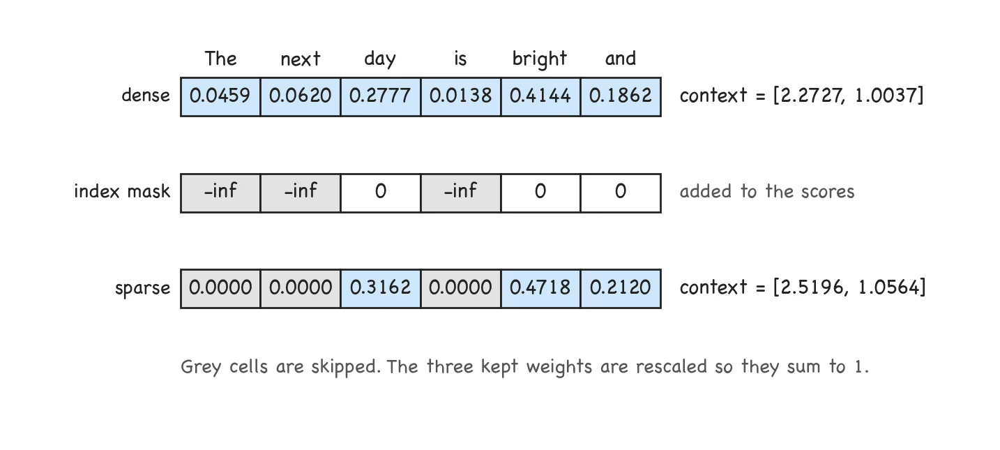
The two vectors are close but not identical. The sparse version gave all of its weight to three tokens, so the 12 percent of weight that dense attention spread over "The", "next" and "is" is gone. The V3.2 report handles this gap by training: the model is trained further with the selection switched on, so its weights adapt to reading only k tokens. That training is the subject of lesson 2.
In this toy example the indexer and the main attention agree on the top three tokens because I chose the numbers that way. In the real model nothing guarantees this at the start. The indexer has to be trained to predict where the main attention puts its weight. That is also lesson 2.
One more detail from the report: the selection is made once per query token, not once per head. DSA uses the MQA mode of MLA, where every head reads the same cached latent entries, so all 128 heads of a query token attend to the same 2,048 tokens.
8. The whole sequence at once
During prefill the model processes all six tokens together, so every row gets its own selection. Running the indexer on all rows with the causal mask gives the pattern in figure 1.7.
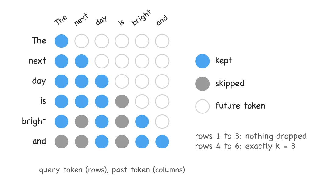
Two things are visible here. The first three rows have at most three candidates, so nothing is dropped: for the first k tokens, sparse attention and dense attention are the same thing. From the fourth row on, every row has exactly k = 3 entries, however long the sequence becomes.
9. How much work is saved
For one new token at context length L, dense attention reads L entries and sparse attention reads k:
L / k = 128,000 / 2,048 = 62.5
For a whole sequence, the first k rows are dense and every later row has k entries:
dense pairs  = L x (L + 1) / 2
sparse pairs = k x (k + 1) / 2 + (L - k) x k
| Toy (L = 6, k = 3) | V3.2 (L = 128,000, k = 2,048) | |
|---|---|---|
| Dense pairs | 21 | 8,192,064,000 |
| Sparse pairs | 15 | 260,047,872 |
| Ratio | 1.4 | 31.5 |
The dense count grows with L squared. The sparse count grows with L x k, and k is fixed. Figure 1.8 plots both counts up to 128,000 tokens.
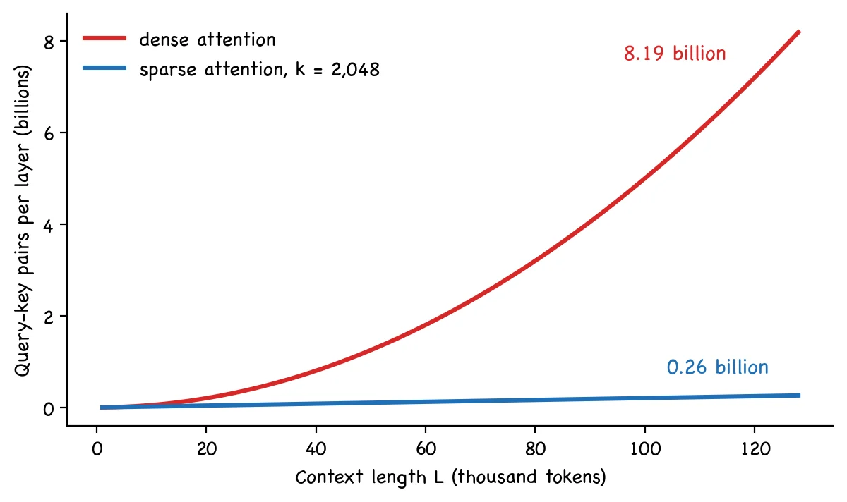
The indexer itself still scores every past token, so its cost grows with L squared as well. The design moves the quadratic part of the work from the expensive module to the cheap one. The report says the indexer needs much less computation than MLA, but it does not give a ratio, so I will not quote one.
10. The indexer in code
The listing below is the indexer function from lesson01_check.py, trimmed to return only the scores and the mask. The script reproduces every table in this lesson.
import torch

def lightning_indexer(H, W_q, W_k, W_w, n_heads, k):
    T = H.shape[0]
    d_i = W_k.shape[1]
    q = (H @ W_q).view(T, n_heads, d_i)                        #A
    keys = H @ W_k                                             #B
    w = H @ W_w                                                #C
    dots = torch.einsum("thd,sd->ths", q, keys)                #D
    scores = (w.unsqueeze(-1) * torch.relu(dots)).sum(dim=1)   #E
    causal = torch.triu(torch.ones(T, T), diagonal=1).bool()
    scores = scores.masked_fill(causal, float("-inf"))         #F
    topk = scores.topk(min(k, T), dim=-1).indices              #G
    index_mask = torch.full((T, T), float("-inf"))
    index_mask.scatter_(-1, topk, 0.0)                         #H
    index_mask = index_mask.masked_fill(causal, float("-inf"))
    return scores, index_mask
#A One small query per token and per indexer head.
#B One small key per token, shared by all indexer heads. This is what gets cached.
#C One weight per indexer head, computed from the query token.
#D Dot product of every query with every key: shape (tokens, heads, tokens).
#E ReLU, then the weighted sum over heads. The result has shape (tokens, tokens).
#F Future tokens can never be selected.
#G The k best past tokens for each query token.
#H The mask the attention layer adds to its scores: 0 for selected tokens, -inf for the rest.
11. What the real model adds
The released V3.2-Exp code follows the same steps, with a few additions that we skipped to keep the arithmetic visible:
- The indexer query is computed from the low-rank query latent of MLA, not directly from the hidden state.
- The indexer keys pass through a LayerNorm.
- Half of the dimensions of each indexer query and key receive RoPE, so the indexer knows about position.
- Queries and keys are rotated with a Hadamard transform and then quantized to FP8 before the dot products. We will cover why a rotation helps quantization when we reach FP4 and FP8.
- The released reference code still computes all attention scores and then adds the mask, as we did in section 7. That shows the correct result but saves no time. The speedup needs an attention kernel that gathers only the selected entries. Kernels come later in this series.
12. What is still open
- How do we train the indexer so that its top k matches where the main attention wants to look? The report uses a KL-divergence loss against the attention weights, in two stages.
- How does the main model adapt to reading only k tokens?
- The indexer is still quadratic in L. DeepSeek-V4 attacks this by compressing the KV entries into blocks before indexing them.
Lesson 2 answers the first two questions with a worked KL example. Lessons 3 and 4 cover the block compression in V4.